Regularization {L1 LASSO} {L2 Ridge}
Description
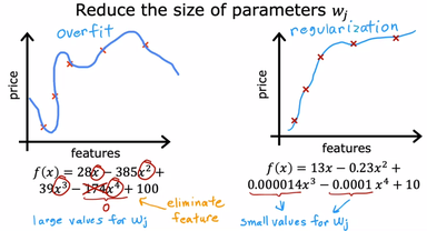
Regularization is a technique used to add a penalty term to the loss function during training. This helps reduce model complexity and prevent overfitting.
There are several types of regularization, including:
- L1 regularization (LASSO)
- L2 regularization (Ridge)
- Elastic net regularization
Varieties
L1 regularization (LASSO - Least Absolute Shrinkage and Selection Operator) is a linear regression technique used for feature selection. It adds a penalty term to shrink less important coefficients to zero, effectively removing them.
LASSO is especially useful for high-dimensional data, where features outnumber samples, helping identify key predictors.
- Advantages: Handles correlated features, performs feature selection and regression simultaneously.
- Limitations: May select only one feature from correlated groups and struggle with very high-dimensional data.
Info
To keep gradient descent from bouncing around the optimum at the end when using lasso regression, you need to gradually reduce the learning rate during training. It will still bounce around the optimum, but the steps will get smaller and smaller, so it will converge.
L2 regularization (Ridge) (Weight Decay), is a technique used to prevent overfitting in machine learning models. It works by adding a penalty term to the loss function, which is proportional to the square of the model's weights.
The penalty term discourages the model from assigning large weights to individual features, leading to a simpler and more generalized model. By minimizing the combined loss function, which includes both the original loss and the penalty term, the model finds a balance between fitting the training data well and keeping the weights small, ultimately improving its ability to generalize to new, unseen data.
Elastic net regression is a middle ground between ridge regression and lasso regression. The regularization term is a weighted sum of both ridge and lasso's regularization terms, and you can control the mix ratio \(r\). When \(r = 0\), elastic net is equivalent to ridge regression, and when \(r = 1\), it is equivalent to lasso regression.
Formula
- \(J(\vec{w}, b)\): Loss function to be minimized.
- \(L(\vec{w}, b)\): Generic loss function (can be MSE, MAE, etc).
- \(\vec{w}\): Model parameters (weights/coefficients).
- \(n\): Number of features (or weights).
- \(\lambda\): Regularization strength.
- \(|w_i|\): Absolute value of the \(i\)-th parameter (\(w_i\)).
- \(J(\vec{w}, b)\): Loss function to be minimized.
- \(L(\vec{w}, b)\): Generic loss function (can be MSE, MAE, etc).
- \(\vec{w}\): Model parameters (weights/coefficients).
- \(n\): Number of features (or weights).
- \(m\): Number of training examples.
- \(\lambda\): Regularization strength.
- \(w_i^2\): Squared value of the \(i\)-th parameter (\(w_i\)).
- \(J(\vec{w}, b)\): Loss function to be minimized.
- \(L(\vec{w}, b)\): Generic loss function (can be MSE, MAE, etc).
- \(\vec{w}\): Model parameters (weights/coefficients).
- \(n\): Number of features (or weights).
- \(m\): Number of training examples.
- \(\lambda\): Regularization strength.
- \(|w_i|\): Absolute value of the \(i\)-th parameter (\(w_i\)). Used in the L1 Norm (Lasso).
- \(w_i^2\): Squared value of the \(i\)-th parameter (\(w_i\)). Used in the L2 Norm (Ridge).
-
\(r\): Mixing parameter for Elastic Net. This value, where \(0 \le r \le 1\), determines the blend between L1 and L2 penalties.
- If \(r=1\), the penalty is purely L1 (Lasso).
- If \(r=0\), the penalty is purely L2 (Ridge).
Workflow
تو تصویر بالا نشون داده شده که با اعمال ضریب های (w) کوچک امتحان میکنیم که آیا حذف یک متغیر دارای توان به حل مشکل ما کمک میکند یا خیر، از آنجایی که مقادیر w و b را سیستم بطور اتوماتیک تعیین میکند و ما در آنها نقشی نداریم لذا با استفاده از روش زیر، سیستم را مجبور به انتخاب اعداد کوچک برای ضریب های (w) دلخواه خود میکنیم:
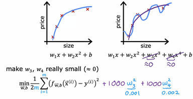
در تصویر بالا ما تنها تاثیر دو متغیر w سه و w چهار را کم کردیم، اما در سیستم های پیچیده تر بجای این کار از الگوی زیر استفاده می شود:
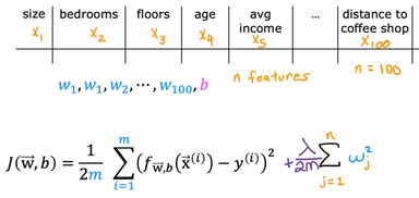
در الگوی بالا n تعداد متغیر های (w) های حاضر در معادله هستش، با بالا بردن \(\lambda\) سیستم مجبور به انتخاب w های کوچکتر می شود که دقیقا هدف ما از انجام Regularization هستش
Example
from sklearn.linear_model import LogisticRegression

# Train logistic regression with L1 (Lasso) penalty
model = LogisticRegression(solver="liblinear", penalty="l1", max_iter=1000)
model.fit(X, y)
from sklearn.linear_model import Ridge

model = Ridge(alpha=1.0)
model.fit(X, y)
from sklearn.linear_model import ElasticNet

model = ElasticNet(alpha=0.1, l1_ratio=0.5)
model.fit(X, y)
Info
l1_ratio corresponds to the mix ratio \(r\)
Vs
- Regularization is generally recommended, even in small amounts, to improve model generalization.
- Ridge regression serves as a reliable default choice for most cases.
- Lasso or Elastic Net are preferable when only a few features are expected to be relevant, as they tend to reduce the weights of irrelevant features to zero.
- Elastic Net is generally favored over Lasso, since Lasso may behave unpredictably when the number of features exceeds the number of training instances or when features are highly correlated.